Introduction
Sequence prediction is one of the hottest application of Deep Learning these days. From building recommendation systems to speech recognition and natural language processing, its potential is seemingly endless. This is enabling never-thought-before solutions to emerge in the industry and is driving innovation. There are many different ways to perform sequence prediction such as using Markov models, Directed Graphs etc. from the Machine Learning domain and RNNs/LSTMs from the Deep Learning domain.
In this article, we will see how we can perform sequence prediction using a relatively unknown algorithm called Compact Prediction Tree (CPT). You'll see how this is a surprisingly simple technique, yet it's more powerful than some very well known methods, such as Markov Methods, Directed Graphs, etc.
I recommend reading this article before going further - A Must-Read Introduction to Sequence Modelling(with use cases). In this, Tavish introduced us to an entirely new class of problems called Sequence Modelling, along with some very good examples of their use cases and applications.
Table of Contents
- Primer about Sequence Prediction
- Compact Prediction Tree Algorithm (CPT)
- Understanding the Data Structures in CPT
- Understanding how training and prediction works in CPT
- Training Phase
- Prediction Phase
- Creating Model and Making Predictions
Primer about Sequence Prediction
Sequence prediction is required whenever we can predict that a particular event is likely to be followed by another event and we need to predict that. Sequence prediction is an important class of problems which finds application in various industries. For example:
- Web Page Prefetching - Given a sequence of web pages that a user has visited, browsers can predict the most likely page that a user will visit and pre-load it. This will, in turn, save time and improve the user experience
- Product Recommendation - The sequence in which a user has added products into his/her shopping list can be used to recommend products that might be of interest to the user
- Sequence Prediction of Clinical Events - Given the medical history of a patient, Sequence Prediction can be leveraged to perform differential diagnosis of any future medical conditions
- Weather Forecasting - Predicting the weather at the next time step given the previous weather conditions.
There are numerous additional areas where Sequence Prediction can be useful.
Current landscape of solutions
To see different kinds of solutions available for solving problems in this field, we had launched the Sequence Prediction Hackathon. The participants came up with different approaches and the most popular of them was LSTMs/RNNs which was used by most of the people in the top 10 on the private leaderboard.
LSTMs/RNNs have become a popular choice for modelling sequential data, be it text, audio, etc. However, they suffer from two fundamental problems:
- They take a long time to train, typically tens of hours
- They need to be re-trained for sequences containing items not seen in the previous training iteration. This is a very costly process and is not feasible for scenarios where new items are encountered frequently
Enter CPT (Compact Prediction Tree)
Compact Prediction Tree (CPT) is one such algorithm which I found to be more accurate than traditional Machine Learning models, like Markov Models, and Deep Learning models like Auto-Encoders.
The USP of CPT algorithm is its fast training and prediction time. I was able to train and make predictions within 4 minutes on the Sequence Prediction Hackathon dataset mentioned earlier.
Unfortunately, only a Java implementation of the algorithm exists and therefore is not as popular among Data Scientists in general (especially those who use Python).
So, I have created a Python version of the library using the documentation developed by the algorithm creator. The Java code certainly helped in understanding certain sections of the research paper.
The library for public usage is present here and you are most welcome to make contributions to it. The library is still incomplete in the sense that it does not have all recommendations of the author of the algorithm, but is good enough to get a decent score of 0.185 on the hackathon leaderboard, all within a few minutes. Upon completion, I believe the library should be able to match the performance of RNNs/LSTMs for this task.
In the next section, we will go through the inner workings of the CPT algorithm, and how it manages to perform better than some of the popular traditional machine learning models like Markov Chains, DG, etc.
Understanding the Data Structures in CPT
As a prerequisite, it is good to have an understanding of the format of the data accepted by the Python Library CPT. CPT accepts two .csv files - Train and Test. Train contains the training sequences while the test file contains the sequences whose next 3 items need to be predicted for each sequence. For the purpose of clarity, the sequences in both Train and Test files are defined as below:
  1,2,3,4,5,6,7
  5,6,3,6,3,4,5
  .
  .
  .
Note that the sequences could be of varying length. Also, One-hot encoded sequences will not give appropriate results. The CPT algorithm makes use of three basic data structures, which we will talk about briefly below.
1. Prediction Tree
A prediction tree is a tree of nodes, where each node has three elements:
- Item - the actual item stored in the node.
- Children - list of all the children nodes of this node.
- Parent - A link or reference to the Parent node of this node.
A Prediction Tree is basically a trie data structure which compresses the entire training data into the form of a tree. For readers who are not aware of how a trie structure works, the trie structure diagram for the below two sequences will clarify things.
Sequence 1: A, B, C
Sequence 2: A, B, D
The Trie data structure starts with the first element A of the sequence A,B,C and adds it to the root node. Then B gets added to A and C to B. The Trie again starts at the root node for every new sequence and if an element is already added to the structure, then it skips adding it again. The resulting structure is shown above. So this is how a Prediction Tree compresses the training data effectively.
2. Inverted Index (II)
Inverted Index is a dictionary where the key is the item in the training set, and value is the set of the sequences in which this item has appeared. For example,
Sequence 1: A,B,C,D
Sequence 2: B,C
Sequence 3: A,B
The Inverted Index for the above sequence will look like the below:
II = { ‘A’:{‘Seq1’,’Seq3’}, ’B’:{‘Seq1’,’Seq2’,’Seq3’}, ’C’:{‘Seq1’,’Seq2’}, ’D’:{‘Seq1’} }
3. LookUp Table (LT)
A LookUp Table is a dictionary with a key as the Sequence ID and value as the terminal node of the sequence in the Prediction Tree. For example:
Sequence 1: A, B, C
Sequence 2: A, B, D
LT = { “Seq1” : node(C), “Seq2” : node(D) }
Understanding how Training and Prediction works in CPT
We will go through an example to solidify our understanding of the Training and Prediction processes in the CPT algorithm. Below is the training set for this example:
| A | B | C | |
| A | B | ||
| A | B | D | C |
| B | C |
As you can see, the above training set has 3 sequences. Let us denote the sequences with ids: seq1, seq2 and seq3. A, B, C, and D are the different unique items in the training dataset.
Training Phase
The training phase consists of building the Prediction Tree, Inverted Index (II), and the LookUp Table (LT) simultaneously. We will now look at the entire training process phase.
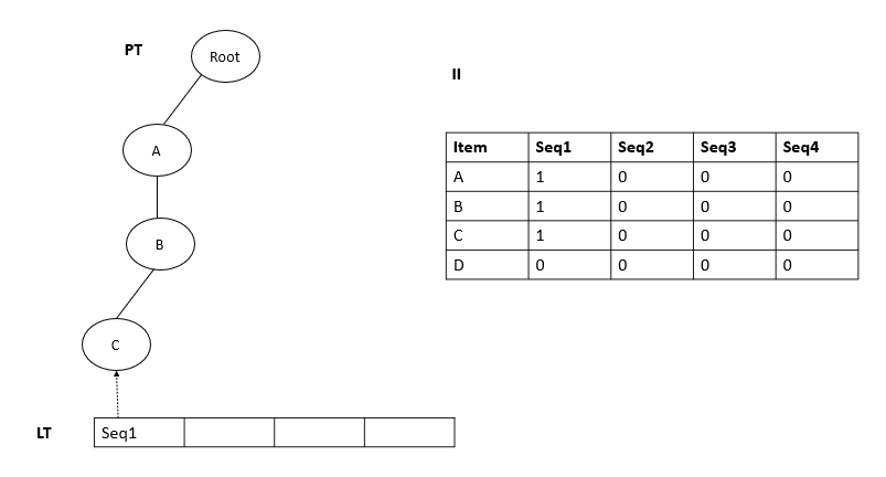
Step 1: Insertion of A,B,C. 
We already have a root node and a current node variable set to root node initially.
We start with A, and check if A exists as the child of the root node. If it does not, we add A to the child list of the root node, add an entry of A in Inverted Index with value seq1, and then move the current node to A.
We look at the next item, i.e B, and see if B exists as the child of the current node, i.e, A. If not, we will add B to the child list of A, add an entry of B in the Inverted Index with value seq1 and then move the current node to B.
We repeat the above procedure till we are done adding the last element of seq1. Finally, we will add the last node of seq1, C, to the LookUp table with key = “seq1” and value = node(C).
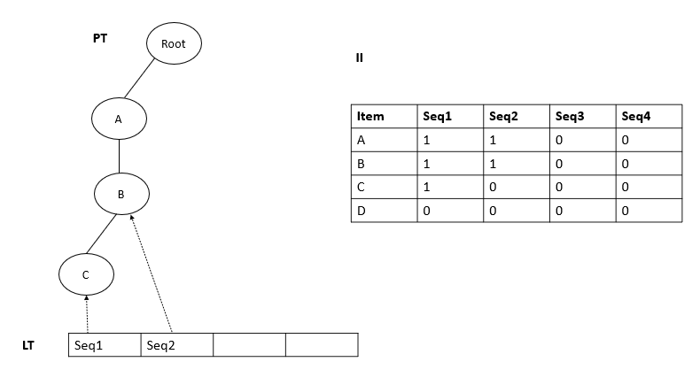
Step 2: Insertion of A,B. 
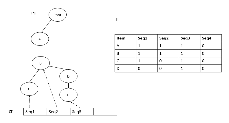
Step 3: Insertion of A,B,D,C. 
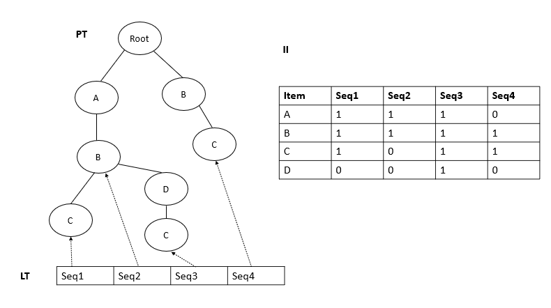
Step 4: Insertion of B,C. 
We do keep doing this till we exhaust every row in the training dataset (remember, a single row represents a single sequence). We now have all the required data structures in place to start making predictions on the test dataset. Let’s have a look at the prediction phase now.
Prediction Phase
The Prediction Phase involves making predictions for each sequence of the data in the test set in an iterative manner. For a single row, we find sequences similar to that row using the Inverted Index(II). Then, we find the consequent of the similar sequences and add the items in the consequent in a Counttable dictionary with their scores. Finally, the Counttable is used to return the item with the highest score as the final prediction. We will see each of these steps in detail to get an in-depth understanding.
Target Sequence - A, B
Step 1: Find sequences similar to the Target Sequence.
Sequences similar to the Target Sequences are found by making use of the Inverted Index. These are identified by:
- finding the unique items in the target sequence,
- finding the set of sequence ids in which a particular unique item is present and then,
- taking an intersection of the sets of all unique items
For example:
Sequences in which A is present = {‘Seq1’,’Seq2’,’Seq3’}
Sequences in which B is present = {‘Seq1’,’Seq2’,’Seq3’,’Seq4’}
Similar sequences to Target Sequence = intersection of set A and set B = {‘Seq1’,’Seq2’,’Seq3’}
Step 2: Finding the consequent of each similar sequence to the Target Sequence
For each similar sequence, consequent is defined as its longest sub-sequence after the last occurrence of the last item of the Target Sequence in the similar sequence minus the items present in the Target Sequence.
** Note this is different from what the developers have mentioned in their research paper, but this has worked for me better than their implementation.
Let's understand this with the help of an example:
Target Sequence = ['A','B','C']
Similar Sequence = ['X','A','Y','B','C','E','A','F']
Last item in Target Sequence = ‘C’
Longest Sub-Sequence after last occurrence of ‘C’ in Similar Sub-Sequence = [‘E’,’A’,’F’] Consequent = [‘E’,’F’]
Step 3: Adding elements of the Consequent to the Counttable dictionary along with their score.
The elements of consequent of each similar sequence is added to the dictionary along with a score. Let's continue with the above example for instance. The score for the items in the Consequent ['E','F'] is calculated as below:
current state of counttable = {}, an empty dictionary
If the item is not present in the dictionary, then,
score = 1 + (1/number of similar sequences) +(1/number of items currently in the countable dictionary+1)*0.001
otherwise,
score = (1 + (1/number of similar sequences) +(1/number of items currently in the countable dictionary+1)*0.001) * oldscore
So for element E, i.e. the first item in the consequent, the score will be
score[E] = 1 + (1/1) + 1/(0+1)*0.001 = 2.001
score[F] 1 + (1/1) + 1/(1+1)*0.001 = 2.0005
After the above calculations, counttable looks like, counttable = {'E' : 2.001, 'F': 2.0005}
Step 4: Making Prediction using Counttable
Finally, the key is returned with the greatest value in the Counttable as the prediction. In the case of the above example, E is returned as a prediction.
Creating Model and Making Predictions
Step 1: Clone the GitHub repository from here.
git clone https://github.com/NeerajSarwan/CPT.git
Step 2: Use the below code to read the .csv files, train your model and make the predictions.
#Importing everything from the CPT file from CPT import *
#Creating an object of the CPT Class model = CPT()
#Reading train and test file and converting them to data and target. data, target = model.load_files(“./data/train.csv”,”./data/test.csv”)
#Training the model model.train(data)
#Making predictions on the test dataset predictions = model.predict(data,target,5,1)
End Notes
In this article, we covered a highly effective and accurate algorithm for sequence predictions - Compact Prediction Tree. I encourage you to try it out yourself on the Sequence Prediction Hackathon dataset and climb higher on the private leaderboard! If you want to contribute to the CPT library, feel free to fork the repository or raise issues. If you know of any other methods to perform Sequence Predictions, write them in the comments section below. And do not forget to star the CPT library. 🙂